Discrete Diffusion Modeling by Estimating the Ratios of the Data Distribution

Overview

Reference: [https://arxiv.org/abs/2310.16834, https://github.com/louaaron/Score-Entropy-Discrete-Diffusion]
https://aaronlou.com/blog/2024/discrete-diffusion/
Why this paper?:diffusion model 을 언어 데이터와 같은 discrete 데이터에 적용하기 위해 diffusion 모델의 기본이론인 score matching을 discrete structure에도 일반화함. empirical 하게 어느정도 성과를 거둠.
Core Question/Purpose: 확산 모델을 언어 데이터에 어떻게 적용할 수 있을까? 기존 auto-regressive 모델과 경쟁할 수 있을까?

Summary

High-Level Summary:
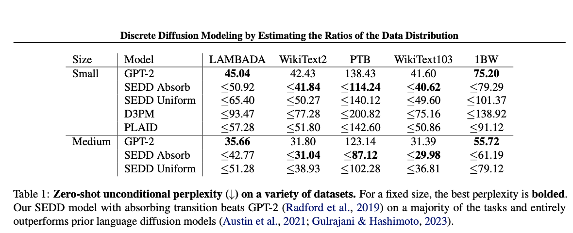
기존의 diffusion model은 자연어와 같은 discrete data에서 성능이 부족함. 이를 해결하기 위해 이 논문에선 기존 diffusion model의 loss인 'Score Entropy'를 discrete space에 일반화하여, Score Entropy Discrete Diffusion(SEDD)를 개발함. SEDD 모델은 기존 language diffusion model 대비 perplexity를 크게 낮추고 GPT-2 수준의 성능을 보임.

auto-regressive 모델이 자연어와 같은 이산 구조 데이터에 전부이고, 더 많은 데이터와 하이퍼 파라미터가 필요하다고 말했지만, 이는, 1. controll(생성과정 중 데이터 분포에서이탈, drift한다.)이 어렵고, 2. inference하면 토큰마다 생성하니 병렬화가 어려우며, 3. 단방향으로 작업이 진행되어, 앞 단어, 뒤 단어가 지정하는 등의 제어를 하기 매우 어렵다. 따라서 SEDD를 제안한다.
에너지 기반 모델의 문제는 Z를 아는 것이 매우매우 어렵다는 것이다.
$p_{θ} (x)$ 를 직접 모델링 하는 대신 $\frac{p_{θ} (y)}{p_{θ} (x)}$ 를 모델링 한다.
이러면 Z 를 제거 가능하니까..
따라서

s_{θ} (x)_{y} \approx \frac{p_{d a t a} (y)}{p_{d a t a} (x)}

이것은 유명한 연속공간 score function $\nabla_{x} l o g p$ 와 categorical equivalent하다. (여기서 motivate 많이됨)
중요하게. 우리는 신경망 근사를 $s_{θ} (x)_{y}$ 로 쓴다. 이때, 하나의 네트워크 평가로 모든 비율 계산이 가능해야한다는 것이다. 이때 분모는 $p_{d} a t a (x)$ 로 고정이다. 가능한 모든 y에 대해 계산하면, $N^{d}$ 개의 항이 생기는 것이기에, relevant ratio만 선택적으로 모델링하고, y가 x와 close 하다고 판단되는 경우에만 선택한다.
이를 $y \sim x$ 라고 함.(그래프이론식 표기. y와 x는 이웃) 여기에서는 한 위치만 다른 문장을 이용함.
Pasted image 20250402133747.png
Cross entropy loss이용

E_{y \sim p_{d a t a}} [- l o g p_{θ} (y)] = - \sum_{y} p_{d a t a} (y) l o g p_{θ} (y)

Score entropy

\sum_{y \sim x} s_{θ} (x)_{y} - \frac{p_{d a t a} (y)}{p_{d a t a} (x)} l o g s_{θ} (x)_{y} $ $! [언 어 모 델 링 데 이 터 분 포 비 율 . g i f] (/ i m g / u s e r / b l o g 로 그 항 덕 분 에 항 상 0 보 다 큼 몬 테 카 를 로 샘 플 링 적 용 하 고, s c o r e m a t c h i n g t e c h q u e 적 용 하 면, $ p_{d a t a} (x) = \sum_{y} p (x | y) p_{0} (y) $ 가 되 고, 따 라 서 d e n o i s i n g s c o r e e n t r o p y l o s s 는 다 음 과 같 음 $ $ E_{x_{0} \sim p_{0}, x \sim p (\cdot | x_{0})} [\sum_{y \sim x} s_{θ} (x)_{y} - \frac{p (y | x_{0})}{p (x | x_{0})} l o g s_{θ} (x)_{y}]

data 분포가 아니라 $x_{0}$ 에 대한 조건부 분포로 만든게 큼.

노이즈란 무엇인가?
연속공간은 가우시안 노이즈 때리지만, 이산공간은 다른 요소를 jump해야함

1. Intro

1.1 Background

text generation 분야에선 auto-regressive model이 경쟁력있는 방법으로 자리 잡고 있음.
하지만, auto-regressive model은 느린 샘플링 속도, 제어의 어려움, 성능 저하로 인한 분포 조정의 필요 등의 한계를 보임.
이미지 도메인에서 성공한 diffusion 모델을 자연어 분야에 적용하려는 시도가 있음.

2. Preliminaries

2.1 Discrete Diffusion Processes

discrete data에 대한 Diffusion Processs는 Continuous time Markov chain으로 정의됨. 이는 diffusion matrix $Q_{t}$ 를 통해 정의됨. $\frac{d p_{t}}{d t} = Q_{t} p_{t} p_{0} \approx p_{d a t a}$
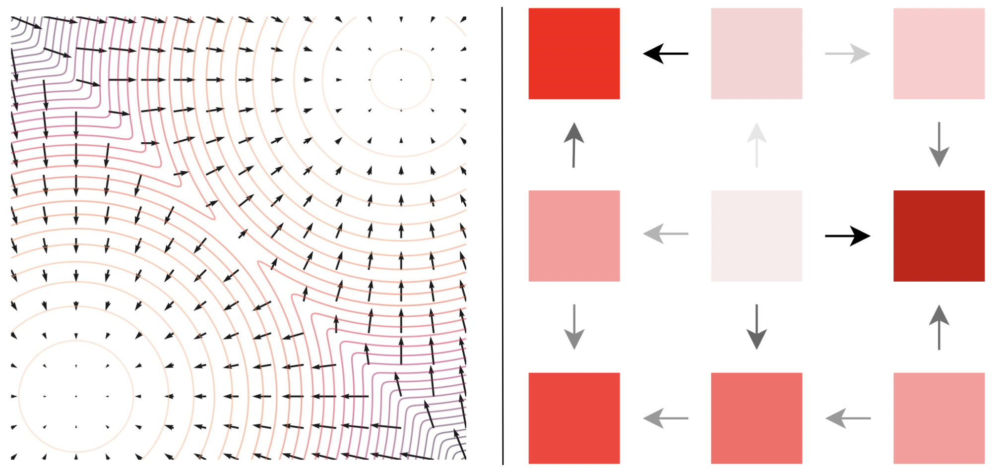
- 이 확산 과정은 아주 작은 $△ t$ 를 이용한 오일러 간격으로 근사하여 시뮬레이션 가능하며, reverse-diffusion matrix는 diffusion matrix의 probablity ratio ( $\frac{p_{t} (y)}{p_{t} (x)}$ )로 정의할 수 있음. 이는 특정 score function $\nabla_{x} l o g p_{t}$ 을 일반화한 것이다.
  
  -이때 discrete structure에서 gradient operator는 $x \neq y$ 인 $x, y$ 로 다음과 같이 정의된다.
  $\nabla f (x y) := f (y) - f (x)$
  score function 은 normalize된 gradient를 일반화한다.
  $\frac{\nabla p (x y)}{p (x)} = \frac{p (y)}{p (x)} - 1$

\frac{d p_{T - t}}{d t} = {\bar{Q}}_{T - t} p_{T - t} {\bar{Q}}_{t} (y, x) = \frac{p_{t} (y)}{p_{t} (x)} Q_{t} (x, y)

{\bar{Q}}_{t} (x, x) = - \sum_{y \neq x} {\bar{Q}}_{t} (x, y)

2.2 Discrete Diffusion Models

discrete diffusion model 은 reverse diffusion 과정에서 데이터 분포의 ratio를 학습하는 것을 목표로 한다.
discrete space에서는 기존 continuous diffusion model에서 사용하던 Score matching이 명확히 확립되지 않아 다양한 방법론이 혼재해있었다.
이제 그것들 분석하고 이론적, 경험적 한계를 지적할거다.

Mean prediction

ratio $\frac{p_{t} (y)}{p_{t} (x)}$ 를 직접적으로 매개변수화 하는 것이 아니라, reverse diffusion dentity $p_{0 | t}$ 를 학습하여 간접적으로 ratio를 얻는다.
objective가 continuous time에서 명확하지 않고 근사가 필요하며, 밀도를 직접학습하는 것은 난이도가 높아, 이 방법은 실제 성능이 크게 낮았다.

Ratio Matching

dimension 별로 marginal probability들을 maximum likelihood 방식으로 학습한다.
이 방법은 표준적인 score matching과 크게 벗어나고, 특별하고 비싼 신경망 구조를 필요로 한다.
결과적으로 Mean Prediction 보다 성능이 떨어진다.

Concrete Score Matching

기존의 Fisher divergence를 일반화한 접근법이다.
이 방법은 probability ratio 근사를 목표로하지만, $\frac{p_{t} (y)}{p_{t} (x)}$ 가 양수여야하는 조건과 $l^{2}$ loss의 불일치로 인해 수렴하지 않는 문제점이 있다.
이론적 배경에도 불구하고 성과가 부족하다.
학습하는 것 : $s_{θ} (x, t) \approx [\frac{p_{t} (y)}{p_{t} (x)}]_{y} \neq x$

L_{C S M} = \frac{1}{2} E_{x \sim p_{t}} [\sum_{y \neq x} (s_{θ} (x_{t}, t)_{y} - \frac{p_{t} (y)}{p_{t} (x)})^{2}]

appendix.D

Concrete score matching 쓴거 GPT2 랑 score entropy랑 비교했는데 likelihood loss 3~4배,
perplexity는 만배 커짐. -> 수렴 잘 안됨.

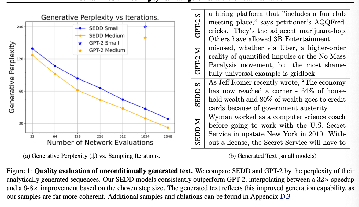
Generative perplexity 평가
D.2. Further Evaluation of Generative Perplexity

We further evaluate our generative perplexity for uniform models as well as different sampling schemes (analytic sampling based on Tweedie’s vs Euler sampling based off of reverse diffusion). Results are shown in Figure 2. Generally, we find that uniform does not produce the same linear tradeoff curve as absorbing (most likely due to a bottleneck in generation quality). Futhermore, analytic generally outperforms Euler sampling, and this is a major factor for the uniform model.

We also generated on our trained baselines (Austin et al., 2021; Gulrajani & Hashimoto, 2023), finding both performed substantially worse than our SEDD Absorb baseline but slightly better than our SEDD Uniform.

Tweedie 이론이랑 Euler 방식 비교
Analytic 방식이 Euler 방식 보다 샘플링 성능(perplexity)가 괜찮았따. 몇가지 모델로도 더 해봤는데, SEDD absorb보다는 성능이 안좋았지만 SEDD uniform 보다는 좋았따.

Score Entropy Discrete Diffusion Models

Score entropy는 Concrete Score Matching과 달리 목표로 하는 probability ratio의 양수 조건을 discrete diffusion 과정에서 만족하도록 설계했다.
$w_{x y}$ 는 0보다 크거나 같고, $s_{θ} (x)_{y}$ 는 score network이다. K(a)는 $a (l o g a - 1)$ 로 $L_{s e}$ 를 0보다 항상 크거나 같게 할 수 있도록 해주는 normalizing constant function이다.

E_{x \sim p} [\sum_{y \neq x} w_{x y} (s_{θ} (x)_{y} - \frac{p (y)}{p (x)} l o g s_{θ} (x)_{y} + K (\frac{p (y)}{p (x)}))]

Fisher Divergence 대신 Bregman divergence를 이용한다.
$D_{F} (s (x)_{y}, \frac{p (y)}{p (x)}) when F = - l o g is convex func$
따라서 non-negative, symmetric, convex하다. 그리고 기존 cross entropy 도 general positive value로 일반화 할 수 있다.

Score Entropy Properties

Score entropy는 ground truth concrete score를 포함하는 적절한(suitable) loss function이다.

$p$ 가 $w_{x y} > 0$ 이고 fully support 된다고 가정해보자. 데이터의 수와 model capacity가 무한하다면, 최적의 파라미터 $θ^{*}$ 는 위 cross entropy를 최소화하고, 다시말해 $s_{θ^{*}} (x)_{y} = \frac{p (y)}{p (x)}$ 를 모든 $x, y$ pair에 대해 만족한다. 그리고 loss는 0이된다.

score entropy는 문제가 되는 gradients를 rescaling 함으로써 concrete score 보다 직접적으로 낫다. $w_{x y} = 1$ , $\nabla_{s_{θ} (x)_{y}} L_{S E} = \frac{1}{s_{θ} (x)_{y}} \nabla_{s_{θ} (x)_{y}} L_{C S M}$ 각 (x,y)쌍의 gradient 신호들은 $s_{θ} (x)_{y}$ 를 마치 normalizing 항으로 이용하듯 scaling된다. 그리고 레전드 디자인 K(log-barrier)가 $s_{θ}$ 를 0이상으로 유지한다.

concrete score matching과 같이 score entropy는 모르는 $\frac{p (y)}{p (x)}$ 를 제거함으로써 계산적으로 다루기 쉽게 만든다. 왜? p(x),p(y)는 데이터 전채를 뜻어봐야하잖아.

$L_{S E}$ 는 $θ$ 에 영향을 안주는 상수항을 제외하면, implicit score entropy와 동일한데,
-$$\mathcal{L}{ISE}=\mathbf E{x \sim p} \bigg [\sum_{y \neq x} w_{xy}s_\theta(x)y - wlog \space s_\theta(x)_y \bigg]$$
근데 이거 몬테카를로 식으로 추정하려면, x 샘플링해서 x당 가능한 모든 y에 대해 $s_{θ} (y)_{x}$ 를 해야한다. 근데 고차에선 이 연산이 비현실적으로 복잡하기에, y를 uniform하게 sampling할 수 밖에 없다. 하지만 이러면 Hutchinson trace estimaotr에서 말한 추가적인 variance 와 유사한 문제가 생기게 된다. 이로 인해 ISE는 대규모 데이터에서는 부적합하다. 따라서 Vincent의 denoising score matching 형태의 변형된 Score Entropy를 이용한다.

Denoising Score Entropy
transition kernal $p (\cdot | \cdot)$ (ie $p (x) = \sum_{x 0} p (x | x_{0}) p_{0} (x_{0})$ )와 base density $p_{0}$ 의 pertubation $p$ 를 가정하자. 이러면 score entorpy는 $θ$ 에 영향 안주는 상수를 제외하면 Denoising score entropy는 다음과 같다.

L_{D S E} = \underset{\begin{matrix} x_{0} \sim p_{0} \\ x \sim p (\cdot ∣ x_{0}) \end{matrix}}{E} [\sum_{y \neq x} w_{x y} (s_{θ} (x)_{y} - \frac{p (y | x_{0})}{p (x | x_{0})} l o g s_{θ} (x)_{y})]

얘는 몬테카를로 샘플링 할때, 하나의 $s_{θ} (x)$ 만 계산하면, $s_{θ} (x) y$ 값이 포함되어있고, $x_{0}$ 으로 생기는 variance는 제어가능하므로 Denoising score entropy는 scalable하다.!

Likelihood Bound For Score Entropy Discrete Diffusion

ELBO를 정의할거임. -> likelihood-기반 학습과 평가에 필요함.

dependent score network $s_{θ} (\cdot, t)$ , parameterized reverse matrix ${\bar{Q}}_{t}^{θ} (y, x)$ =

s_{θ} (x, y)_{y} Q_{t} (x, y) w h e n, x \neq y, - \sum_{z \neq x} {\bar{Q}}_{t}^{θ} (x, y) w h e n, x = y

그리고 parameterized densities $p_{t}^{θ}$ 는 다음 식을 만족.

\frac{d p_{T - t}^{θ}}{d t} = {\bar{Q}}_{T - t}^{θ} p_{T - t}^{θ} p_{T}^{θ} = p_{b a s e} \approx p_{T}

diffusion 그리고 forward probabilities가 위에 구해졌으므로...

- l o g p_{0}^{θ} (x_{0}) <= L_{D W D S E} (x_{o}) + D_{K L} (p_{T | 0} (\cdot | x) | | p_{b a s e})

여기서 $L_{D W D S E}$ 는 diffusion weighted denoising score entropy임.

식으로는. $L_{D W D S E} =$

\int_{0}^{T} E_{x_{t} \sim p_{t | 0} (\cdot | x_{0})} \sum_{y \neq x_{t}} Q_{t} (x_{t}, y) (s_{θ} (x_{t}, t)_{y} - \frac{p_{t | 0} (y | x_{0})}{p_{t | 0} (x_{t} | x_{0})} l o g s_{θ} (x_{t}, t)_{y} + K (\frac{p_{t | 0} (y | x_{0})}{p_{t | 0} (x_{t} | x_{0})}))

DWDSE 디자인 해설
Remark. The DWDSE (and the implicit version) can be derived from the general framework of Benton et al. (2022) assuming a concrete score parameterization. In particu- lar, the implicit version coincides with the likelihood loss introduced in Campbell et al. (2022).

그리고 얘는 고차원 task 에서도 유지됨.
$p_{t | 0}^{s e q} (\hat{x} | x)$ 를 각 토큰 별 joint distribution으로 표현가능 함.
우리가 $Q_{t}^{t o k} = σ (t) Q^{t o k}$ 로 설정했기 때문에 모델링 야무지게 가능.

근데 문제는 Q는 확산과정이므로, $\hat{x}$ 만큼 존재하는데 이건 Austin(Structured denoising diffusion models in dis- crete state-spaces)과 Campbell(A continuous time framework for discrete denoising models)의 이전 작업으로 처리. 두개의 standard matrix를 이용. MASK abosorbing state와 완전히 연결된 그래프구조로부터 소개된 것.
Pasted image 20250408135521.png

4. Simulating Reverse Diffusion with Concrete Scores

Campbell(A continuous time framework for discrete denoising models)에 $τ$ -leaping 적용
given a sequence $x_{t}$ .

δ_{x_{t}^{i}} (x_{t - Δ t}^{i}) + Δ t Q_{t}^{t o k} (x_{t}^{i}, x_{t - Δ t}^{i}) s_{θ} (x_{t}, t)_{i, x_{t - Δ t}^{i}}

근데 $s^{θ}$ 가 true concrete을 잘 학습했는지는 알 수 없음(agnostic). 특히 모든 $\frac{p_{t} (y)}{p_{t} (x)}$ 를 모두 알아야 Tweedie's theoremTweedie’s formula and selection bias과 유사한 형태를 만들수있음.

$p_{t}$ 가 diffusion ODE $d p_{t} = Q p_{t}$ 를 따른다고 하면,
true denoiser는

p_{0 | t} (x_{0} | x_{t}) = (e x p (- t Q) [\frac{p_{t} (i)}{p_{t} (x_{t})}]_{i = 1}^{N})_{x 0} e x p (t Q) (x_{t}, x_{0})

근데 모든 ratio 모르고ㅗ 오직 Hamming distance 가 1인 시퀀스만 파악할 수 있기 때문에 token transition probabilities를 다음과 같이 작성함.(for $x_{t - Δ t}^{i}$ )

(e x p (- σ_{t}^{Δ t} Q) s_{θ} (x_{t}, t)_{i})_{x_{t - Δ t}^{i}} e x p (- σ_{t}^{Δ t} Q) (x_{t}^{i}, x_{t - Δ t}^{i})

w h e r e σ_{t}^{Δ t} = (\bar{σ} (t) - \bar{σ} (t - Δ t

(Tweedie τ-leaping). Let
$p_{(t - Δ t | t)}^{t w e e d i e} (x_{t - Δ t} | x_{t})$ 가 위 식의 token update rule의 확률이라고하자. KL divergence를 최소화하는 $s_{θ}$ 가 완벽히 학습되었다면, 모든 $τ$ -leaping strategies에 있어서 true인 $p_{(t - Δ t | t)} (x_{t - Δ t} | x_{t})$ 이다.

그리고

Pasted image 20250408142706.png

결과

Pasted image 20250408142737.png

Pasted image 20250408142747.png
Pasted image 20250408142755.png
Pasted image 20250408142809.png